Introduction
ParamRF provides a declarative modelling interface that compiles RF models, such as circuit models, using JAX. This page provides in introduction into how such models are created, and an overview of the fitting procedures.
Core Concepts
The library revolves around a few key building blocks:
pmrf.Model: The base class for any computable RF component. Model methods such as s, a can be used to define model S-parameters, ABCD-parameters etc. and all accept frequency as input. On the other hand, __call__ can be overridden to return a model instance itself. Models can be defined using composition such as cascading existing models, or via inheritance of the model class itself.pmrf.Parameter: A parameter in a model, storing its value as well as any parameter metadata. This allows for parameter bounds and scaling, provides the ability to mark parameters as fixed, and can have a prior associated with it for Bayesian fitting.pmrf.Frequency: A wrapper around a JAX array that defines the frequency axis over which models are evaluated.
Model Composition
ParamRF provides a small component library with commonly-used models such as lumped and distributed elements. Models can be built directly using these in a compositional approach.
Cascaded Models
For simple circuit element chains, the ** operator can be used to cascade several models together.
The example below creates an RLC filter and terminates it in an open circuit. The resultant rlc is a first-class Model of type pmrf.models.containers.Cascade, consisting of parameters representing the respective R, L and C parameters. The S11 is then plotted using matplotlib.
import pmrf as prf
from pmrf.models import Resistor, Inductor, ShuntCapacitor, OPEN
from pmrf.parameters import Fixed

# Instantiate the lumped element models
resistor = Resistor(R=100.0, name="res")
inductor = Inductor(L=2e-9)
capacitor = ShuntCapacitor(C=1e-12)

# Cascade the models, storing the result, and a terminated version with fixed R
rlc = resistor ** inductor ** capacitor
terminated_rlc = rlc.terminated(OPEN).with_params(res_R=Fixed(90.0))

# Plot the S11 of the terminated model directly using matplotlib
import matplotlib.pyplot as plt
freq = prf.Frequency(1, 1000, 1000, 'MHz')
s11 = terminated_rlc.s_db(freq)[:,0,0]
plt.plot(freq.f_scaled, s11)
Circuit Models
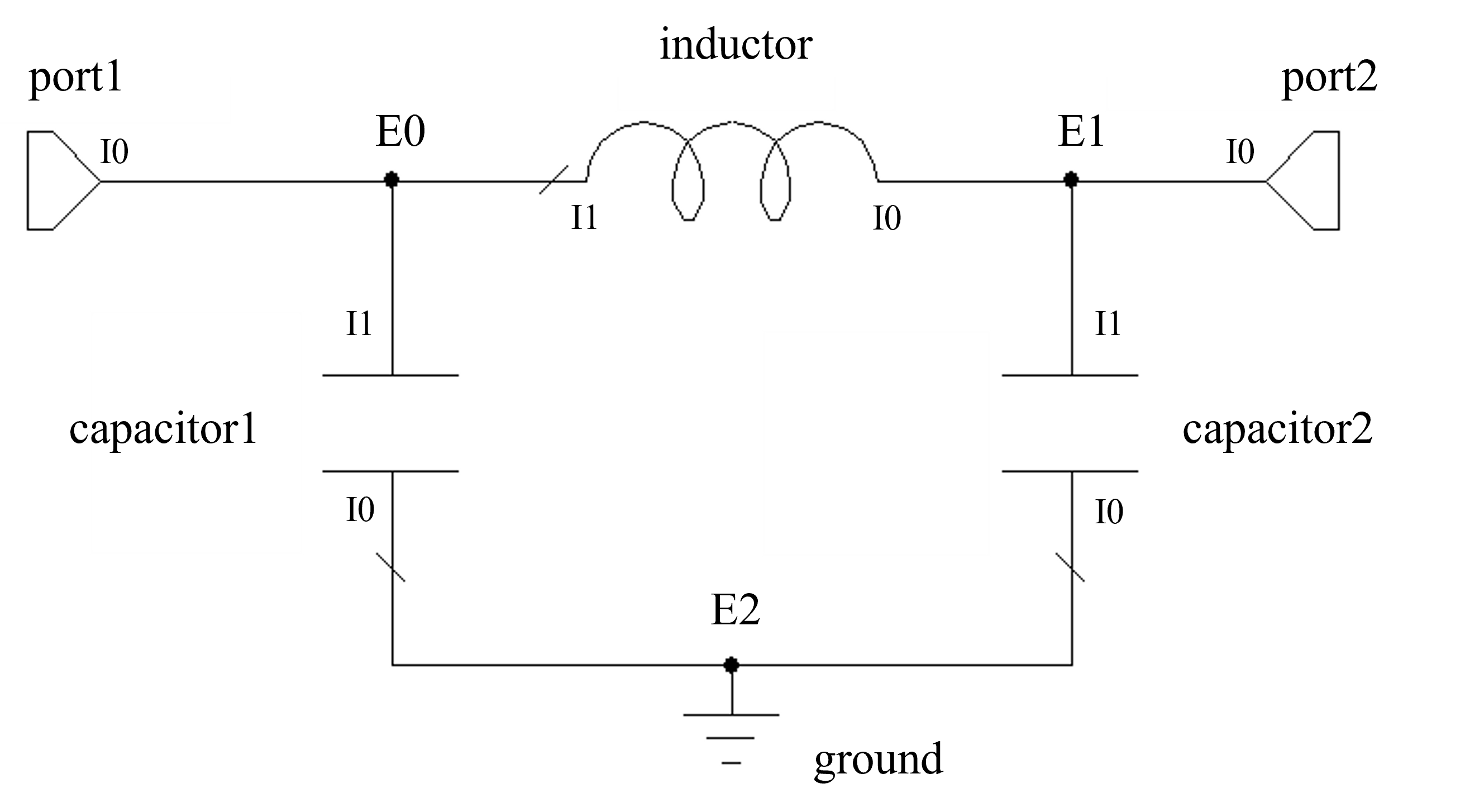
For complex circuits, ParamRF offers the ability to combine models in any desired configuration using the Circuit class. This class accepts a list of “connections”. Each entry in this list is a node in the circuit. Each node is another list, with each element being a tuple for each connected circuit element or sub-model. Each tuple then contains the model object, as well as the index of the port for that model that is connected in that node.
The following example uses this method to define a two-port PI-CLC network. “External” nodes (each entry in the outer list) are numbered as E0, E1 etc. whereas “internal” port indices (ports for each model in the circuit) are numbered per element as I0, I1 etc. The model is then converted to a scikit-rf network and plotted.
import pmrf as prf
from pmrf.models import Capacitor, Inductor, Circuit, Port, Ground

# Instantiate the elements, ports and grounds
capacitor1, capacitor2 = Capacitor(C=2e-12), Capacitor(C=1.5e-12)
inductor = Inductor(L=3e-9)
port1, port2 = Port(), Port()
ground = Ground()

# Create the connections list
connections = [
    [(port1, 0), (capacitor1, 1), (inductor, 1)], # E0
    [(port2, 0), (capacitor2, 1), (inductor, 0)], # E1
    [(ground, 0), (capacitor1, 0), (capacitor2, 0)], # E2
]

# Create the model and convert it to a scikit-rf Network at a desired frequency, ploting S21
pi_clc = Circuit(connections)
pi_clc_skrf = pi_clc.to_skrf(prf.Frequency(1, 1000, 1001, 'MHz'))
pi_clc_skrf.plot_s_db(m=0, n=0)
Model Inheritance
For more complex models (such as equation-based ones), users can inherit directly from the Model class and override one of the network properties (such as s, a, or y) or the __call__ method.
Any attributes of a model are classified as either static or dynamic. By default, fields of built-in types such as str, int, list etc. are seen as static in the model hierarchy, whereas those annotated as a Parameter or Model are dynamic and can be adjusted (for example, by fitting routines).
Note that parameter initialization is flexible: parameters may be populated with a simple float value; using factory methods such as Uniform, Normal or Fixed; or directly using the Parameter class constructor.
Equation-based Models
The following example demonstrates custom model definition by defining a capacitor from first principles. This could be used, for example, to implement more complex analytic or surrogate models. Here, one of the typical network properties, such as s, a, y etc., must be overriden, returning the resultant matrix directly.
import jax.numpy as jnp
import pmrf as prf

# Define a model class. Behaviour is defined by implementing
# a primary matrix function such as "s" in this case.
class Capacitor(prf.Model):
    C: prf.Parameter = 1.0e-12

    def s(self, freq: prf.Frequency) -> jnp.ndarray:
        w = freq.w
        C = self.C

        z0_0 = z0_1 = self.z0
        denom = 1.0 + 1j * w * C * (z0_0 + z0_1)
        s11 = (1.0 - 1j * w * C * (jnp.conj(z0_0) - z0_1) ) / denom
        s22 = (1.0 - 1j * w * C * (jnp.conj(z0_1) - z0_0) ) / denom
        s12 = s21 = (2j * w * C * (z0_0.real * z0_1.real)**0.5) / denom

        return jnp.array([
            [s11, s12],
            [s21, s22]
        ]).transpose(2, 0, 1)
Circuit Models
Sometimes it is still convenient to inherit from Model while still building the model using cascading or Circuit. In this case, the model can be built from sub-models fields/attributes, and returned by overriding the __call__ method.
The following example creates a PI-CLC model once again, but using the above method. Note how certain parameters can be given initial parameters, bounds or fixed to a constant (useful for fitting).
import jax.numpy as jnp
import pmrf as prf
from pmrf.models import Capacitor, Inductor, Circuit, Port, Ground
from pmrf.parameters import Uniform, Fixed

class PiCLC(prf.Model):
    capacitor1: Capacitor =     Capacitor(C=Fixed(1.0e-12))
    capacitor2: Capacitor =     Capacitor(C=Uniform(0.0, 10.0, value=2.0, scale=1e-12))
    inductor: Inductor =        Inductor(L=Uniform(0.0, 10.0, value=2.0, scale=1e-12))

    def __call__(self) -> prf.Model:
        # Instantiate the ports and grounds
        port1, port2, ground = Port(), Port(), Ground()

        # Create the connections list. This time, capacitor1, capacitor2 and inductor are members.
        connections = [
            [(port1, 0), (self.capacitor1, 1), (self.inductor, 1)], # E0
            [(port2, 0), (self.capacitor2, 1), (self.inductor, 0)], # E1
            [(ground, 0), (self.capacitor1, 0), (self.capacitor2, 0)], # E2
        ]

        # Return the model
        return Circuit(connections)
Fitting
The primary application of pmrf is the fitting of models and their parameters to measured data. The pmrf.fitting module provides a unified interface to perform this task using either traditional frequentist optimization, or Bayesian inference techniques.
The general workflow consists of defining a model, loading data via scikit-rf, and configuring and running the fitter with the specified settings.
Main Fitters
SciPyMinimizeFitter: Provides access to gradient-based and gradient-free optimization algorithms fromscipy.optimize. This includes algorithms such as SLSQP, Nelder-Mead and L-BFGS.PolyChordFitter: Enables Bayesian inference through nested sampling. This approach provides maximum likelihood parameter values, as well as full posterior probability distributions and Bayesian evidence useful for model comparison and uncertainty quantification.
Fitting Example
The following provides a complete example of fitting the built in CoaxialLine model to the measurement of 10m coaxial cable (provided as an example in the GitHub). Data is loaded using scikit-rf; the model is instantiated with appropriate initial parameters; the fitter is configured with a custom cost function and subsequently run; and results are plotted.
import matplotlib.pyplot as plt
import logging
import skrf as rf
import jax.numpy as jnp

from pmrf.models.lines import CoaxialLine
from pmrf.parameters import Uniform, Fixed, PercentNormal
from pmrf.fitting import SciPyMinimizeFitter
from pmrf.functions import l2_norm_ax0, mag_2_db

logging.basicConfig(level=logging.INFO)

# Load the measured data and setup the model
measured = rf.Network('data/10m_cable.s2p', f_unit='MHz')
model = CoaxialLine(
    din = PercentNormal(1.12, 5.0, scale=1e-3),
    dout = PercentNormal(3.2, 5.0, scale=1e-3),
    epr = PercentNormal(1.45, 5.0, n=2),
    rho = PercentNormal(1.6, 5.0, scale=1e-8),
    tand = Uniform(0.0, 0.01, value=0.0, scale=0.01, n=2),
    mur = Fixed(1.0),
    length = PercentNormal(10.0, 5.0),
    epr_model='bpoly',
    tand_model='bpoly',
)

# Initialize the fitter. We fit on the real and imaginary and combine their results
fitter = SciPyMinimizeFitter(
    model=model,
    features=['s11_re', 's11_im'],
    cost_function=[l2_norm_ax0, jnp.sum, mag_2_db],
)

# Run the fit
results = fitter.fit(measured, optimizer='Nelder-Mead')
model_ntwk = results.fitted_model.to_skrf(measured.frequency)

# Plot some results
fig, axes = plt.subplots(2, 2)
axes = axes.flatten()
model_ntwk.plot_s_db(m=0, n=0, ax=axes[0])
measured.plot_s_db(m=0, n=0, ax=axes[0])
model_ntwk.plot_s_deg(m=0, n=0, ax=axes[1])
measured.plot_s_deg(m=0, n=0, ax=axes[1])
model_ntwk.plot_s_re(m=0, n=0, ax=axes[2])
measured.plot_s_re(m=0, n=0, ax=axes[2])
model_ntwk.plot_s_im(m=0, n=0, ax=axes[3])
measured.plot_s_im(m=0, n=0, ax=axes[3])

plt.show()
Sampling
A secondary application of pmrf is the random sampling or simulation of models using e.g. Latin Hypercube sampling.
The below example demonstrates a very simple example of simulating 10 different resistor networks with uniform resistance between 9 and 11 ohms.
import pmrf as prf
from pmrf.models import Resistor
from pmrf.parameters import Uniform
from pmrf.sampling import LatinHypercubeSampler

resistor = Resistor(R=Uniform(9.0, 11.0))
sampler = LatinHypercubeSampler(resistor)
resistors = sampler.generate_models(10)
freq = prf.Frequency(10, 20, 100, 'MHz')

for i, res in enumerate(resistors):
    res.export_touchstone(freq, f'resistors_{i}')